Extreme Spread groups
The accuracy of a batch of ammunition is determined by shooting a number of groups, with a fixed number of shots in each group. The distance between the two shots furthest apart in each group is measured - these are the so called extreme spreads of the groups. An average of these extreme spreads is calculated and that average, or "mean", of the extreme spreads is then a measure of the quality of the ammunition.

The value of the extreme spread will vary from group to group in a random way. The more groups that are shot, the more accurate the mean of the extreme spreads will be. The accuracy of the mean of the measured extreme spreads will depend in a predictable way on the number of groups fired and the number of shots in each group. See the Group Statistics article on this website.

Measuring Extreme Spread groups
A statistical analysis of Extreme Spread groups assumes a centre-to-centre measurement of the two shot holes furthest apart in the groups. But it is usually much easier to measure the position of the edge of a shot hole, where there is a sharp transition from paper to hole, than the centre of the hole itself.

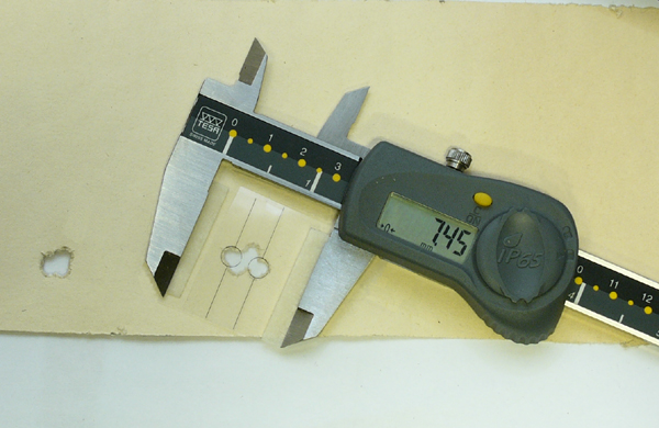
Too, the inner edge of the furthest separated shot holes may be obliterated by other shots in the group, making an estimation of the centres of the two shot holes of interest more difficult. So, frequently (mostly) it is the outside-edge-to-outside-edge that is measured. Extreme Spread Edge to Edge (ESEE) measurements can be converted to Extreme Spread Centre to Centre (ESCC) measurements simply by deducting the bullet diameter from the ESEE results.

In the picture below, the graticules taped to the jaws of the calipers are printed on overhead-projector type transparency film. It is relatively easy to use Photoshop, or some similar image software, to create a .222" diameter circle set into a vertical line, which is then printed off onto the transparency film. When taping the graticules to the caliper jaws, the circles and lines need to accurately overlap each other. The nice thing about electronic calipers is that they can be zeroed for that particular jaw separation when the graticules are taped in place. The circles can be used to measure 'Centre to Centre' extreme spreads and the vertical lines to measure 'Edge to Edge' extreme spreads.

Group Shape
The tacit assumption when using the Extreme Spread method is that the shape of the group is round and that the scatter in the group is purely random. In real life, this is not always the case - the groups often have a systematic elongation in some direction. Such an elongation will be rifle related, not ammunition related, so can usually be fixed so that the elongation is reduced or eliminated and the size of the consequent round groups will be purely down to random dispersion in the ammunition. Even vertical dispersion due to variation in the velocity of the ammunition (see the Velocity Dispersion article on this website), which might be considered an ammunition problem, can be nullified by "tuning" the rifle.

The problem is that a simple measurement of the extreme spread of a group will not reveal any systematic elongation in the groups. Other measurements need to be made to tease out the non-roundness in the group shape. One way forward is to measure the Extreme Spread Angle (ESA), which is the angle to the horizontal (say) of a line drawn through the two extreme spread shots. Vertically strung groups will have Extreme Spread Angles varying around a Mean Extreme Spread Angle (MESA) of 90 degrees, and the standard deviation of the ESAs around the MESA will be quite small.

One problem with measuring ESAs is shown up when horizontal groups are considered. The ESAs of the individual groups will vary around zero degrees. But because groups with angles between 180 and 360 degrees are effectively indistinguishable from those with angles between 0 and 180 degrees, the result will be two ESA distributions, one clustered just above 0 degrees and the other clustered just below 180 degrees, as represented by the two bottom groups on the right. Moreover, the MESA for horizontal groups will be 90 degrees - the same as for vertical groups! And basically round groups, with ESAs spread evenly between 0 and 180 degrees, will also have a MESA of 90 degrees.

The connundrum is solved when looking at the standard deviations for the various types of groups. Basically round groups, with ESAs spread evenly between 0 and 180 degrees, will have standard deviations of about 55 degrees. Vertical groups with some degree of linearisation or elongation will have standard deviations less than 55 degrees. The more elongated the basic group shape is, the smaller the standard deviation on ESAs will be. Because circular groups are the most random, the standard deviation cannot be greater than 55 degrees. If the calculated standard deviation of the ESAs turns out to be greater than 55 degrees, the basic group is horizontally elongated and is being represented by two separate distributions, some near 0 degree and some near 180 degrees.

The final solution is to measure the Extreme Spread Angle for each group to the horizontal and to the vertical. If the basic group shape is circular, or vertical, or horizontal, the MESA will be around 90 degrees for both horizontal and vertical ESAs. For circular groups, the standard deviations will be around 55 degrees for both sets of results. For horizontal groups, the ESA standard deviation will be greater than 55 degrees for the ESA results measured against a horizontal line, so use standard deviation for the ESAs against the vertical line. Groups laying at some angle between the vertical and horizontal will have standard deviations which are very similar in both sets of results, and MESAs which differ by about 90 degrees.

The protractor shown to the left is contrived so that the vertical and horizontal ESA of a group can both be measured with one setting of the protractor. In this example, the ESA is 41 degrees to the horizontal, and 131 degrees to the vertical. Clicking on the image gives a hi-res version of the protractor which can be printed out on an overhead projector type transparancy, then cut out for use.