|
Introduction
The most quoted work on the statistics of groups is "Statistical Measures of Accuracy for Riflemen and Missile Engineers" by Frank E. Grubbs, Ph.D., (November 1964. Another edition was published in 1991). This monograph was privately published, so copies of it are not easily available. In this monograph, Grubbs evaluates all the commonly used methods of determining accuracy by measurement of group size - and then some. Grubbs' analysis shows that the most efficient means of determining the accuracy of ammunition from a given number of rounds down the range, is the Radial Standard Deviation method, defined as, "...the square root of the total sum of squares of the deviations in the x and y directions from their respective sample means, divided by the number of points of impact." However, this involves plotting the position on an x-y grid of every shot fired, which experimentally is a time consuming procedure. Too, any paper target would have to be changed frequently to ensure each shot left an individual bullet hole. Ordnance factories which use this method of quality testing for their ammunition will usually have an electronic target system which records the fall of shot automatically on an x-y grid. But such electronic target systems are prohibitively priced.
But the Extreme Spread method is not so efficient as the Radial Standard Deviation method. More shots down the range are needed to get the same level of certainty about the accuracy of the ammunition. Too, there is the problem about how many shots to fire in each group. If you fire too few shots in each group, the centre of each group is poorly known. A tight looking group may in fact be a statistically rare small cluster of shots well separated from what would be the centre of a much larger group if more shots were fired. Now, with the Extreme Spread method, the size of each group is determined by just two shots, irrespective of the number of shots in the group. Even if two hundred shots were fired in each group, only two shots would determine the group size and the other 198 shots would have (almost) no contribution to make. So, while the centre of a group with such a large number of shots in it is fairly well defined, (that is the contribution of the other 198 shots), the random nature of the two shots that determined the group size mean that the next 200 shot group will have a different size from the first one. A lot of bullets will go down the range before a meaningful average of a 200 shot group size is known! For Extreme Spread groups then, maximising the efficiency (how well the average group size can be determined from a given number of shots) is a balancing act between how well the group centre is known (a lot of shots in the group) against the average contribution of each shot to determining the group size (just a few shots in each group).
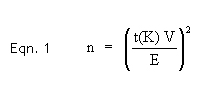
Statistical analysis Using the well known sample size equation, let n be the number of groups you need to shoot. Let E be the level of inaccuracy in the average group size you are prepared to tolerate (10% in this case) and let K be the confidence level that you need (90% in this case). Then:-
The term V in this equation is the "Coefficient of Variation", which is equal to the standard deviation on the variation of group size, divided by the mean group size. These two quantities can only really be determined experimentally. Actually shooting groups is one way to do it, but running Monte Carlo numerical simulations on a computer is cleaner, cheaper and a lot quicker and Grubbs publishes the results of "shooting" one thousand groups in a computer. An abreviated table of these results is given below. (Values given are in terms of the total population standard deviation, which was the average distance from the centre of the group of all the shots fired in the 1000 groups.)
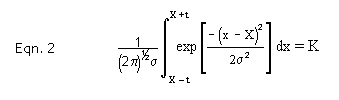
The term t(K) is the confidence level expressed in terms of standard deviations for a Gaussian curve, where:-
K is the confidence level required, 2X is the mean value of the group size and sigma is the population standard deviation. The area under the normalised Gaussian curve between the limits of t either side of the mean is equal to the confidence level. Any book on statistics thicker than a postcard will have tables of t verses K. Table 2 below gives a few values that will be handy.
Now the questions posed above can be answered. When shooting five shot groups, say, the Coefficient of Variation V is equal to the variation in group size, which is 0.824 from Table 1 above, divided by 3.067, which is the mean value from the table. Thus V = 0.269. What this means is that for five shot groups, the size of the groups will vary by about 27% on average, from group to group. From Table 2, the value of t(K) is 1.65 for a confidence level K of 90% The term E, the tolerated error in the mean group size value, is expressed as a straight percentage of unity. For a 10% error then, E = 0.1 Plugging these values into equation 1 above, the result is that n = 19.7 or, rounding to the nearest whole number, 20 groups are required to get a mean value that is within 10% of the actual value, with a 90% confidence level. The total number of shots down the range will be 5 times 20 or 100 shots. For an error of only 5% of the mean value and a confidence level of 95%, the number of shots down range rises to 550!
Grouping efficiency
One interesting point to note is how fast the number of shots required climbs as the as the tolerated error is reduced. An error of 10% with a confidence level of 90% will cost a couple of boxes of ammunition. Just halve that error and the ammo required is measured in bricks, not boxes. The lesson to learn is that for any practical testing of ammunition, trying to obtain error levels better than 10% is very costly in terms of time and ammunition. At least 300 rounds down the range would be required for the error in the measured average group size to be much less than 10%. The other point of interest is that the most efficient number of shots to shoot in a group is seven. The number of shots tabulated in Table 3 is rounded up or down so the numbers correspond to complete groups, which means the results are a little lumpy. But as the tolerated error decreases and the number of shots grows, the quantization of the group number has less effect and the seven shot group starts to stand out as the most efficient. Seven shots in a group is the best balance between knowing where the centre of the group is and the average contribution of each shot to the measured size of the group. It is common to shoot five shot groups and it can seen that shooting five shot groups is almost as efficient as seven shot groups. Ten shot groups is a little worse than five shot groups and 3 shot groups is worse yet. As for 20 shot or more groups - a waste of good ammo. Given that rimfire ammo comes in boxes of 50, which is neatly laid out in rows of 5, shooting five shots groups would appear to be the best balance of practicality and efficiency. It should be noted here that the first mention (to my knowledge) that the most efficient number of shots in a group for the Extreme Spread method is seven, was by G.Sitton in the "Handloader" magazine, (September-October 1990, starting page 42) who communicated a statistical analysis by Ken Kees and Dr. Banister of Speer Bullets.
|
 Practically, the Extreme Spread method the easiest to use. A number of groups are shot on paper, each group having a certain number of shots. For each group, the distance between the two shots furthest apart in the group is measured. It does not then matter then if all the shots fall into a "one hole" group, it is the largest diameter of that hole that is of interest. The average of these extreme spreads of all the groups fired is then a measure of the quality of the ammunition. For the back yard ballistician, the Extreme Spread method is far and away the most popular method used.